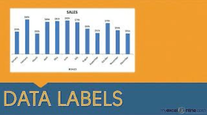
44 how to add multiple data labels in excel
How to Add Data Labels to an Excel 2010 Chart - dummies On the Chart Tools Layout tab, click Data Labels→More Data Label Options. The Format Data Labels dialog box appears. You can use the options on the Label Options, Number, Fill, Border Color, Border Styles, Shadow, Glow and Soft Edges, 3-D Format, and Alignment tabs to customize the appearance and position of the data labels. Add or remove data labels in a chart Right-click the data series or data label to display more data for, and then click Format Data Labels. Click Label Options and under Label Contains, select the Values From Cells checkbox. When the Data Label Range dialog box appears, go back to the spreadsheet and select the range for which you want the cell values to display as data labels.
how to insert lines in excel between data In Excel 2019, Excel 2016 and Excel 2013, adding a trend line is a quick 3-step process: Click anywhere in the chart to select it. Select Add Level, and choose the Agent column. T

How to add multiple data labels in excel
How to group (two-level) axis labels in a chart in Excel? (1) In Excel 2007 and 2010, clicking the PivotTable > PivotChart in the Tables group on the Insert Tab; (2) In Excel 2013, clicking the Pivot Chart > Pivot Chart in the Charts group on the Insert tab. 2. In the opening dialog box, check the Existing worksheet option, and then select a cell in current worksheet, and click the OK button. 3. microsoft excel - Multiple data points in a graph's labels ... add Data Labels > Inside Base for the whole chart add a 2nd series based on the Label column (via right-click Select Data... > Add, do not change Axis Labels at this stage) - all values will be 0 because it is a text column delete the original Percent-only labels Adding rich data labels to charts in Excel 2013 ... To add a data label in a shape, select the data point of interest, then right-click it to pull up the context menu. Click Add Data Label, then click Add Data Callout . The result is that your data label will appear in a graphical callout. In this case, the category Thr for the particular data label is automatically added to the callout too.
How to add multiple data labels in excel. Add a label or text box to a worksheet You can add labels to forms and ActiveX controls. Add a label (Form control) Click Developer, click Insert, and then click Label . Click the worksheet location where you want the upper-left corner of the label to appear. To specify the control properties, right-click the control, and then click Format Control. Add a label (ActiveX control) How to Create Mailing Labels in Word from an Excel List Your labels are now connected with your worksheet. Step Four: Add Mail Merge Fields to the Labels. Now it's time to add your mail merge fields in Word's labels. Select the first label, switch to the "Mailings" tab, and then click "Address Block." In the "Insert Address Block" window that appears, click the "Match Fields" button. Plot Multiple Data Sets on the Same Chart in Excel ... Follow the below steps to implement the same: Step 1: Insert the data in the cells. After insertion, select the rows and columns by dragging the cursor. Step 2: Now click on Insert Tab from the top of the Excel window and then select Insert Line or Area Chart. From the pop-down menu select the first "2-D Line". Add a DATA LABEL to ONE POINT on a chart in Excel Steps shown in the video above: Click on the chart line to add the data point to. All the data points will be highlighted. Click again on the single point that you want to add a data label to. Right-click and select ' Add data label ' This is the key step! Right-click again on the data point itself (not the label) and select ' Format data label '.
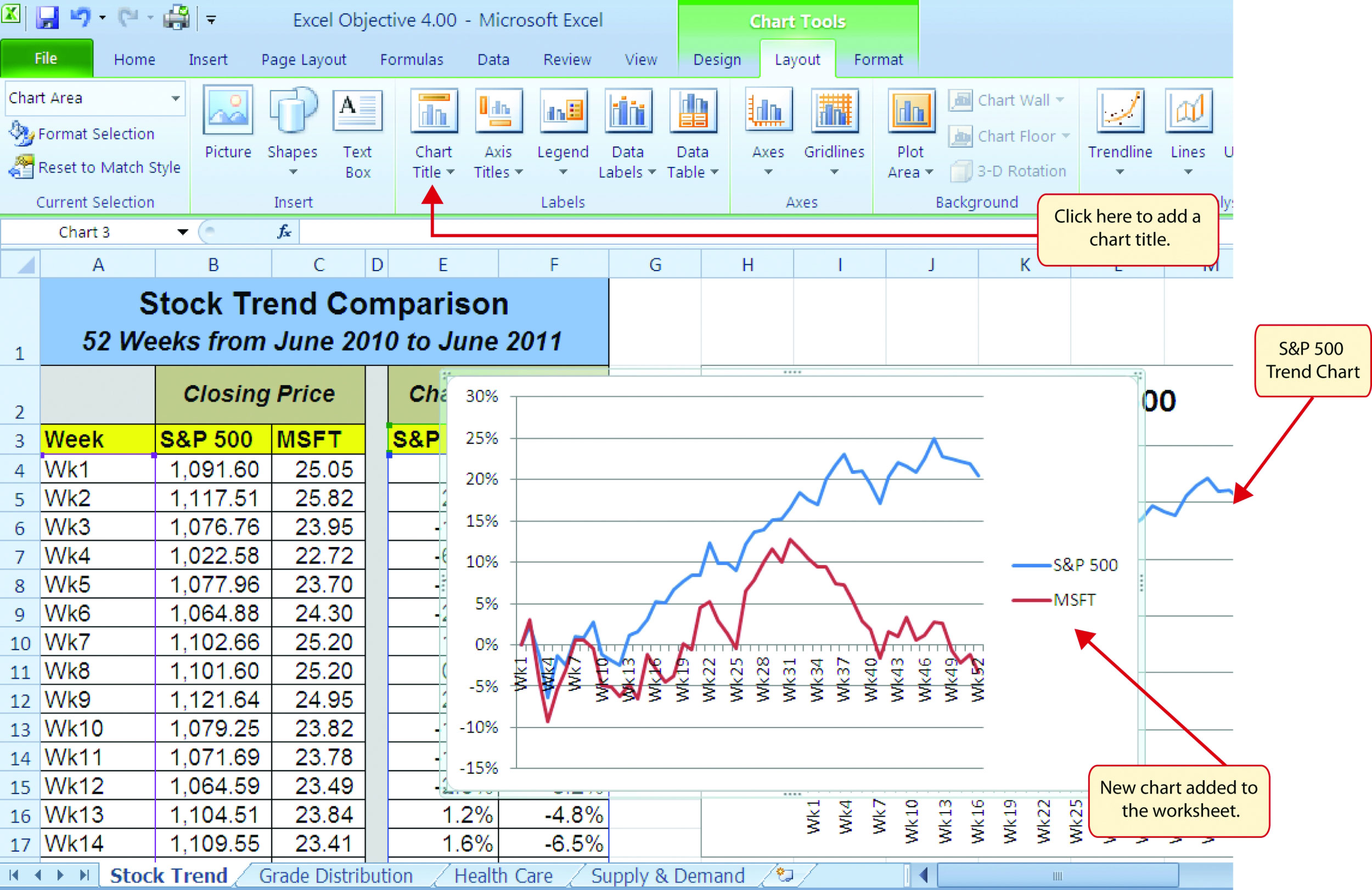
Creating & Labeling Small Multiple Bar Charts in Excel ... Step 4: Add data labels. Ok. This is the section that inspired this post and I am really excited about it. I have been making small multiple bar charts for years. During that time I have been manually dragging the data labels to the outside of the bars. How to Create Multi-Category Charts in Excel ... Step 1: Insert the data into the cells in Excel. Now select all the data by dragging and then go to "Insert" and select "Insert Column or Bar Chart". A pop-down menu having 2-D and 3-D bars will occur and select "vertical bar" from it. Select the cell -> Insert -> Chart Groups -> 2-D Column Bar Chart Insertion Multi-Category Chart How to make row labels on same line in pivot table? Kutools for Excel: a handy add-in with more than 300 advanced tools solves your 90% puzzels in Excel. Make row labels on same line with PivotTable Options You can also go to the PivotTable Options dialog box to set an option to finish this operation. How to Create a Graph with Multiple Lines in Excel | Pryor ... Click Select Data button on the Design tab to open the Select Data Source dialog box. Select the series you want to edit, then click Edit to open the Edit Series dialog box. Type the new series label in the Series name: textbox, then click OK.
Add data labels and callouts to charts in Excel 365 ... Step #1: After generating the chart in Excel, right-click anywhere within the chart and select Add labels . Note that you can also select the very handy option of Adding data Callouts. Step #2: When you select the "Add Labels" option, all the different portions of the chart will automatically take on the corresponding values in the table ... How to add data labels from different column in an Excel ... Right click the data series in the chart, and select Add Data Labels > Add Data Labels from the context menu to add data labels. 2. Click any data label to select all data labels, and then click the specified data label to select it only in the chart. 3. Multi Level Data Labels in Charts - Beat Excel! A better approach is to format modify your data make multiple levels of labels before generating your chart. This way your chart will look much more professional. You don't need to make anything else. After modifying your data, just select all data as you did before and insert your chart. How To Add Axis Labels In Excel [Step-By-Step Tutorial] Axis labels make Excel charts easier to understand.. Microsoft Excel, a powerful spreadsheet software, allows you to store data, make calculations on it, and create stunning graphs and charts out of your data.. And on those charts where axes are used, the only chart elements that are present, by default, include:
Creating Pie Chart and Adding/Formatting Data Labels (Excel) - YouTube
How to create label cards in Excel - Ablebits Click the Create Cards icon in the Transform group on the Ablebits Tools tab: The Create Cards dialog window will appear: By default, the add-in highlights the entire data range in your worksheet. You can select any other range or enter it using your keyboard. Click the Expand selection icon to have the entire table highlighted automatically.

Common Tasks: Chart | Intro | Jan's Working with Numbers
Change the format of data labels in a chart To get there, after adding your data labels, select the data label to format, and then click Chart Elements > Data Labels > More Options. To go to the appropriate area, click one of the four icons ( Fill & Line, Effects, Size & Properties ( Layout & Properties in Outlook or Word), or Label Options) shown here.
Adding Data Labels To An Excel Chart | Free Microsoft Excel Tutorials
How to add or move data labels in Excel chart? To add or move data labels in a chart, you can do as below steps: In Excel 2013 or 2016. 1. Click the chart to show the Chart Elements button . 2. Then click the Chart Elements, and check Data Labels, then you can click the arrow to choose an option about the data labels in the sub menu. See screenshot: In Excel 2010 or 2007

Advanced Graphs Using Excel : fitting curve in excel
How to create Custom Data Labels in Excel Charts Add default data labels Click on each unwanted label (using slow double click) and delete it Select each item where you want the custom label one at a time Press F2 to move focus to the Formula editing box Type the equal to sign Now click on the cell which contains the appropriate label Press ENTER That's it.

How to Make Charts and Graphs in Excel | Smartsheet
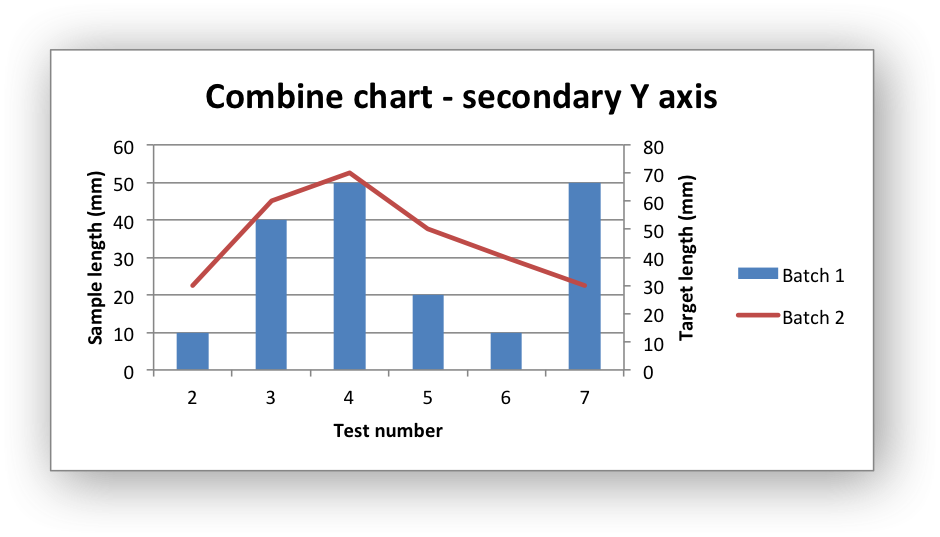
Multiple data labels (in separate locations on chart) Re: Multiple data labels (in separate locations on chart) You can do it in a single chart. Create the chart so it has 2 columns of data. At first only the 1 column of data will be displayed. Move that series to the secondary axis. You can now apply different data labels to each series. Attached Files 819208.xlsx (13.8 KB, 263 views) Download
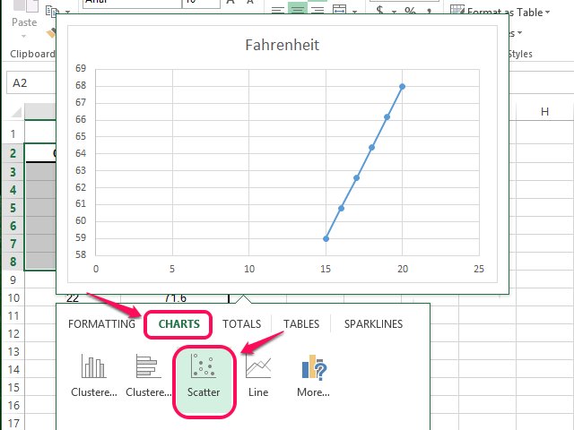
How to Make an XY Graph on Excel | Techwalla.com
How can I add data labels from a third column to a ... Highlight the 3rd column range in the chart. Click the chart, and then click the Chart Layout tab. Under Labels, click Data Labels, and then in the upper part of the list, click the data label type that you want. Under Labels, click Data Labels, and then in the lower part of the list, click where you want the data label to appear.

30 How To Add Label To Excel Chart - Labels Database 2020
How to Customize Your Excel Pivot Chart Data Labels - dummies To add data labels, just select the command that corresponds to the location you want. To remove the labels, select the None command. If you want to specify what Excel should use for the data label, choose the More Data Labels Options command from the Data Labels menu. Excel displays the Format Data Labels pane.

30 What Is A Data Label In Excel - Labels Database 2020
how to add data labels into Excel graphs — storytelling ... You can download the corresponding Excel file to follow along with these steps: Right-click on a point and choose Add Data Label. You can choose any point to add a label—I'm strategically choosing the endpoint because that's where a label would best align with my design. Excel defaults to labeling the numeric value, as shown below.

Format Data Labels in Excel- Instructions | Microsoft excel, Microsoft, Bar chart
Add / Move Data Labels in Charts - Excel & Google Sheets ... Adding Data Labels Click on the graph Select + Sign in the top right of the graph Check Data Labels Change Position of Data Labels Click on the arrow next to Data Labels to change the position of where the labels are in relation to the bar chart Final Graph with Data Labels
Choosing a Chart Type
Adding rich data labels to charts in Excel 2013 ... To add a data label in a shape, select the data point of interest, then right-click it to pull up the context menu. Click Add Data Label, then click Add Data Callout . The result is that your data label will appear in a graphical callout. In this case, the category Thr for the particular data label is automatically added to the callout too.

Do My Excel Blog: How to design a multiple clustered bar chart series in Excel
microsoft excel - Multiple data points in a graph's labels ... add Data Labels > Inside Base for the whole chart add a 2nd series based on the Label column (via right-click Select Data... > Add, do not change Axis Labels at this stage) - all values will be 0 because it is a text column delete the original Percent-only labels
Example: Combined Chart — XlsxWriter Documentation
How to group (two-level) axis labels in a chart in Excel? (1) In Excel 2007 and 2010, clicking the PivotTable > PivotChart in the Tables group on the Insert Tab; (2) In Excel 2013, clicking the Pivot Chart > Pivot Chart in the Charts group on the Insert tab. 2. In the opening dialog box, check the Existing worksheet option, and then select a cell in current worksheet, and click the OK button. 3.

How to Add Data Labels in Excel - Excelchat | Excelchat
EXCEL Charts: Column, Bar, Pie and Line

Excel 2013 Tutorial Formatting Data Labels Microsoft Training Lesson 28.6 - YouTube

How to set and format data labels for Excel charts in C#
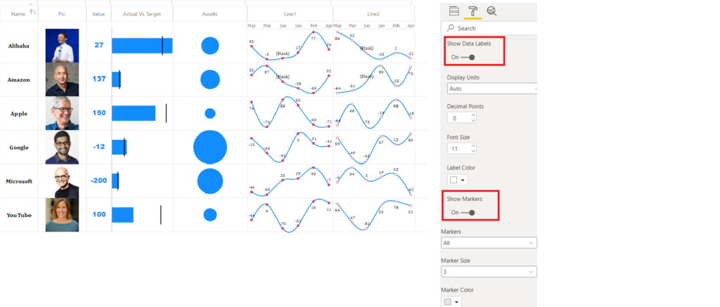
Multiple Sparklines – Power BI & Excel are better together

E-xcel Tuts: Add Data Labels to Excel Charts
Post a Comment for "44 how to add multiple data labels in excel"